Since a camera uses a lens to focus an image to its sensor, lens distortions can be observed. For spherical lenses, there are two common types: Barrel Distortion and Pin Cushion Distortion. Here are the examples for each kind (c/o imagetrendsinc.com):


The aim would be to invert the transformation in order to obtain our ideal image. Two image properties will be corrected in the process: the pixel locations, and their respective graylevel values.
We start by expressing x'=r(x,y) and y'=s(x,y), where r and s are the transformation functions used to map the ideal image to the distorted image frame. It is good to assume that these functions take the form of bilinear functions, r(x,y) = c1*x+c2*y+c3*xy+c4 and s(x,y) = c5*x+c6*y+c7*xy+c8.
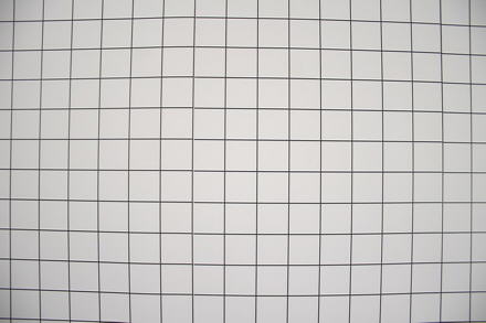
That's basically the physics of this activity as the rest of the steps would make use of matrix manipulations. First, I obtained a barrel-distorted image from imatest.com and cropped it to get this image:

After obtaining the pixel coordinates for the ideal image, we then solve for the coefficients c1 to c8 by setting up the following matrices for each square (thus making the procedure similar to a moving averages run):

We start by expressing x'=r(x,y) and y'=s(x,y), where r and s are the transformation functions used to map the ideal image to the distorted image frame. It is good to assume that these functions take the form of bilinear functions, r(x,y) = c1*x+c2*y+c3*xy+c4 and s(x,y) = c5*x+c6*y+c7*xy+c8.
That's basically the physics of this activity as the rest of the steps would make use of matrix manipulations. First, I obtained a barrel-distorted image from imatest.com and cropped it to get this image:

It's cropped for two reasons: one, this activity aims to demonstrate the concepts used in geometric distortion correction and thus a large grid is not advisable; two, since Scilab works faster with small matrices or images. Notice that the centered square on the grid features the least amount of distortion and our ideal grid was generated from the dimensions of that square. Here are the pixel locations of the points of intersection of the distorted and ideal grids respectively:


and solving for the coefficients using the following equations:


Once the coefficients are obtained, we get the corresponding pixel locations from our distorted image using the set of transformation equations listed above (x' = r(x,y) = c1*x+c2*y+c3*xy+c4 and y' = s(x,y) = c5*x+c6*y+c7*xy+c8) and map out these pixel coordinates to the ideal image map. For the points in the ideal image plane with no corresponding point from the distorted image, we use interpolation methods (bilinear or nearest neighbor) to obtain their grayscale values. Since I practically patterned out my interpolation routine from Gilbert's source (by the way, Gilbert helped me to get this thing working after we consulted Mandy several times), please refer to his source for the interpolation part.
Here are the results I obtained from this activity:


Here are the results I obtained from this activity:


The images above are for the original image, the bilinearly-interpolated image and the image for nearest neighbor interpolation. Although the image was not fully restored, the bilinearly-interpolated image has better quality than the nearest neighbor-interpolated image.

Once again, I'd like to acknowledge Gilbert and Mandy for helping me in getting my version of the source to work. I'm getting a 9 for this activity.. minus one for the delay but 9 for finishing it anyway.


No comments:
Post a Comment