それでいいですか? (Activity # 3)

We were oriented with the different kinds of images today:
1. Binary - simply black and white images
2. Grayscale - shades of gray; where a pixel is given a value between 0 (black) and 255 (white)
3. True-color - has three color channels (usually in RGB)
4. Indexed - similar to true-color except it contains both the image and indexed RGB info.. it is safe to assume that most grayscale images are indexed.

We were asked to collect different types of images.. I selected four pictures, one for each basic type.

Binary

(My own generated image--same as Activity # 2)

FileName: activity_3.bmp
FileSize: 12864
Format: BMP
Width: 320
Height: 320
Depth: 8
StorageType: indexed
NumberOfColors: 2
ResolutionUnit: centimeter
XResolution: 28.340000
YResolution: 28.340000

Grayscale

(This is a picture from the Azusa Nakano Fanclub.)

FileName: 100720.jpg
FileSize: 70426
Format: JPEG
Width: 204
Height: 600
Depth: 8
StorageType: indexed
NumberOfColors: 256
ResolutionUnit: inch
XResolution: 72.000000
YResolution: 72.000000

True-color (the one here is in JPEG.. BMP is not web-friendly)

(Adding the Mahou Shoujo Lyrical Nanoha emblem makes me the final author of this image. If it interests anyone, I got the original background from moe.imouto.org)

FileName: nanoha_wallpaper.bmp
FileSize: 768056
Format: BMP
Width: 640
Height: 400
Depth: 8
StorageType: truecolor
NumberOfColors: 0
ResolutionUnit: centimeter
XResolution: 78.720000
YResolution: 78.72000

Indexed

(Just so you wouldn't think that I prefer 2-D girls over 3-D.. xD I got this fine picture of my favorite seiyuu and J-Pop artist, Mizuki Nana, from Sankaku Complex's Seiyuu Idol Gallery)

FileName: isisuke_uljp01368.png
FileSize: 46755
Format: PNG
Width: 300
Height: 240
Depth: 8
StorageType: truecolor
NumberOfColors: 256
ResolutionUnit: centimeter
XResolution: 117.720000
YResolution: 117.720000

[Edit: Included part b of the activity.]

Unfortunately, Activity # 3 does not end here. What's left to do is to use the area calculation routine in Activity # 2 for a scanned image in Activity # 3. A scanned image is used so that we can have a sense of its physical area, and compare this area with the one obtained using the Green's Theorem.

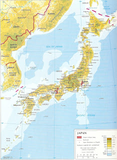
I got the image of Japan from my old volumes of Grolier's Encyclopedia of Knowledge (1999, Vol. 10, p. 316, JAPAN article.) What I did next was to lasso the Hokkaido part of the map, and paint black on a another layer. I removed the layer with the original map, and it left me with a black object on a white background. Then, I inverted the colors to get the second image, and had my contour follower perform the routine to get the last image to the right.

Now here comes the part where I give the details, enough to give the reader an information overload. Wiki tells me that Hokkaido has a land area of 77,981.87 km². The map was drawn to a scale of 1:10,615,000--proper conversion tells me that 1mm in the map is 10,615,000km in physical units (this was confirmed with the use of a ruler xD). The image was scanned to a resolution of 200 dots per inch. Now all that's left to do is the math:

Hehe.. getting that formula to fit the length of this blog site was rather tricky. In any case, the area calculation routine gave me 18691.5 pixels. Now, if were to compare this to our theoretical value, we realize that we have an error of 56%. Why that large of an error? Simply because the routine's weakness is concave curvatures, something that can be quite prominent to an outline of an island.

Oh well, at least the contour follower gave me one hell of an outline. It almost looks like the original pattern. If there's one thing we can learn from this, it's the fact that this area estimation routine has its limits and that more can be done to actually fine-tune its estimation.

P.S. I think I'll have to settle for a ROMANIZED title for my blog post. Will change it the moment I get home. CSRC computers don't have IME. T_T [Edit: Done!] [Edit: Added the imfinfo descriptions.. xD]

The only trick here is to make sure that the filename points to the file and to make sure the file extensions are there. Yey! I get another 10. xD

答えは、どこですか？ (Activity # 2)

[Edit: Prepared this for tomorrow.. that way the title for the post is in Japanese. xD]

We've been having difficulties with siptoolbox here at the CSRC--meaning this activity is post-poned until prior notice.

For now, we've been instructed to generate an image for Activity 2. I came up with this one:


The geometric shape in the binary image needs to be of known area, thus I generated a 320px x 320px image. I cut it diagonally in half, and flipped the inner triangle to obtain the image. Since the image can be reduced to a triangle of half the area of a 320px x 320px square, the area is simply:

320*320 = 102400*0.5 = 51200 square pixels

Apparently, we needed two more images, and here they are:


I set my convention to obtaining the area of the black-shaded regions. The are of the image at the left is simply the area of a triangle of length and base equal to 160px:

0.5*160 px*160 px = 12800 square pixels

Thus, the area of the image at the right is simply equal to half the area of the image subtracted by the area of the inner triangle:

51200 square pixels - 12800 square pixels
= 38400 square pixels

In order to compute for the experimental values, I used the function follow() found on the SIP toolbox. The important chunk of code to use would be:

image = gray_imread('activity_2c.bmp');
for i=1:320, j=1:320; image(i,j)=(image(i,j)*-1)+1; end;
[x,y]=follow(image);

and in order to compute the area, we use Green's Theorem:

n=length(x);
A=0;
for i=1:n-1;
Ai=0.5*(x(i)*y(i+1)-x(i+1)*y(i));
A=A+Ai;
end;

I have Neil to thank for checking my codes. In any case, here are the results:


I used this routine for plotting the follow contours:

xset('window',1)
xbasc()
plot2d(x,y,rect=[0,0,320,320]);

It is important to note that contour assumes the object to be white and its background black. Also, the routine cannot detect any shapes inside a contour, thus making it effective only for contours with defined edges. The area calculated via Green's Theorem yielded the following results:

Image A (unaltered) = 63521 [theoretical: 51200, error: 24.1%]
Image A (sum of B and C) = 50602 [theoretical: 51200, error: 1.17%]
Image A (difference of B and C) = 50840.5 [theoretical: 51200, error: 0.702%]
Image B = 12680.5 [theoretical: 12800, error: 0.934%]
Image C = 37921.5 [theoretical: 38400, error: 1.25%]

I get a 10 for making sure that follow() follows the contour I wanted. xD

AP１８６, 始まります。 (Activity # 1)

The first activity for Physics 186 is Digital Scanning. Nope, the title might seem too simple but it doesn't end there--it's all about reconstructing images.

We started the activity by looking for some old, rugged hand-drawn plots in some old journals in the library last Tuesday. I picked Figure 11 from H. FESHBACH and E.L. LOMON's Boundary Condition Model of Strong Interactions (MIT, Cambridge), ANNALS of PHYSICS: 29, 19-17 (1964).

We had our plot scanned, and received it through e-mail about a night ago. Today, I started with some cropping and rotating tasks, letting loose my obsessive-compulsive. I figured that I'd have a harder time with it, if I don't crop it in the best way I can now.

After cropping, I loaded the image in paint and took note of the XY locations for the ticks (in pixels) on each of the axes. After which, I noted the XY locations for the points (also in pixels). I used OpenOffice.org Calc for storing my data.

I solved for the difference in the actual physical values and divided it by the difference in the X locations of two ticks. I repeated the procedure for the y-ticks and got the scaling factor needed for the points. I obtained a scaling factor of 0.38 for X and -0.04 for Y.

My actual physical position for the points was computed using : 400+[0.38*(x-value for points)] for X and for Y, 40+[-0.04*(y-value for points)]. Note that an initial value of 400 for X and 40 for Y were applied in order to meet the intercepts of the original plot.

What comes next would be the standard way of plotting XY scatter plots c/o Calc. Nothing special really. I believe that getting the area filled by the original plot would take my reader's attention. In itself, it's not special as well. After all, it's in the Help File (to quote, xD) :

Bitmap
Fills the selected object with the bitmap pattern that you click in the list. To add a bitmap to the list, open this dialog in OpenOffice.org Draw, click the Bitmaps tab, and then click Import.

I autoscaled my plot to make sure that the original image remains unaltered while I tinkered with my plot dimensions. I looked for the best values for my XY dimensions for the plot, added the Axes Titles, and poof! I got a plot that looks just like the image at the right.

Not bad for a first activity. It's actually really challenging to get those points to meet once the AUTOFIT feature is used. Not only can't you use the offset options (the ones you get when TILED is enabled), you also get stubborn sizing options for the Chart Area. But yeah, considering you already know how to do it, it'll probably be done in a matter of minutes. ^_^

I'm definitely getting a 10 for this one. xD

新しいサイト?! 無図化して。。 0_0

Is this my new blog site? Nah.

This blog site was specifically made in partial fulfillment to the requirements for my Applied Physics 186 class.

It says here in the syllabus that 'Your blog report will contain all the outputs you produce from this course which include, but are not limited to, graphs, images and results, write-ups from short activities, etc.'

To those who knew of my real blog site, keep it to yourselves. xD

こんにちわ世界?!

Who'd have thought this in itself would get a Wikipedia Article? Hmm.. As far as I can remember, I know of a few ways to do this..

Easiest would be in Python or BASIC:
print "Hello World."

In C it would be something like:
main() {
printf("Hello World.");
}

In FORTRAN, it can either be:
write (*,*) 'Hello World.'
or
print ('a') 'Hello World.'

Oh well.. so much for a sanity test to make sure everything's working.. But when it comes right down to it, it's not such a bad chunk of code to learn. xD