「ai sp@ce」 のバイトは、どうしますか? (Activity # 17)

This activity focuses on photometric stereo, a method of extracting shape and surface detail from shadows. Using this method, we are able to reconstruct an image with surface detail from a series of several images taken at different point sources.

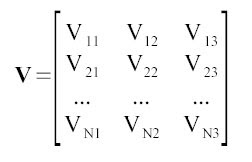
Suppose we have the matrix V given by

where the first index of V represents the image while the second index refers to x, y, and z coordinate of the light source respectively. Assuming these sources illuminate a common object of interest, we can obtain a series of images with intensities defined by

for each point (x,y). We would then have to find g for each point using the usual matrix operation (i.e. inv(V'*V)*V'*I) and normalize the g's to obtain the value for the normal vectors. We get the surface normals using

and finally, we obtain the surface elevation at a point (u,v) using

Following the steps I listed above, here's the Scilab output for the images contained in Photos.mat

I'd like to give myself a 10 for this activity, since this is one of the RARE activities that anyone can finish in one meeting. xD

一番大切なものは? (Activity # 16)

Neural networks is the third classification method for pattern recognition explored in this course, and is the title of activity 16. Unlike the LDA, neural networks don't need heuristics and recognition rules for classification and instead makes use of learning, a function it tries to imitate from the neurons in our brain.

In any case, the activity makes use of the ANN toolbox (ANN_toolbox_0.4.2 found on Scilab's Toolboxes Center) which makes the activity more of a plug-and-play kind of activity.

So how do neural networks work? Each input connection to the artificial neuron has its own weight (synaptic strength) and is multiplied to the inputs, xi. A neuron receives weighted inputs from other neurons and lets the sum act on an activation function g. The result z is then fired as an output to other neurons.

A neural network is formed through the connection of neurons. A typical network consists of an input layer, a hidden layer and an output layer. Just like the previous activities, two modes were considered -- a training mode and a test mode. The parameters one can play around with for the functions in ANN would be the Neural Network architecture (how many neurons for each layer), the Learning Rate and the Number of Iterations.

Using the same data I used in Activity # 15

I had to do a few modifications. First, the inputs must be in a [2xN] matrix (done by transposing the bin after an fscanfMat() call), afterwhich the values must be normalized (ranging from 0 to 1). For the training set, I also had to change the classification values (1 and 2) to 1 and 0 (this is crucial to avoid having erroneous outputs). Finally, here's the output of my neural net classification after round():

For the win, I give myself a pat at the back and a well-deserved 10. xD I'd like to thank Gilbert for his help in helping me understand the ANN toolbox.

好き? (Activity # 15)

Activity # 15 is pretty much like the previous activity except for a little improvement--this time, it uses probabilisitic classification to minimize the risk or loss in classification.

Since my classes can be linearly separated (i.e. one can separate one from the other by drawing a line in the plot in the previous activity), the method I used was Linear Discriminant Analysis, the details of which can be found here.

This time, we were asked to sort out an image with patterns that are close to being similar, i.e. they should have little to no difference. I generated another image of blobs using Photoshop--the blobs are one brush size apart in terms of size and a difference of 50 ticks when it comes to G-channel color value.

Of course, the script is pretty much plug and play.. all that was needed was to obtain data using the script from the previous activity, dump them into an outfile, get the LDA script (found in the tutorial but implemented in scilab) to organize and process the files, and poof! we have an LDA plot as shown above.

Note that unlike the previous activity, it organized all the data points in a line, and that the discriminant functions were successful in classifying close patterns by increasing the difference between them (note the order of magnitude - xE+06). As expected from the image, the LDA results to a perfect classification (100% correct). I'm not sure about real life images though. I'll probably give it a shot when I find some time.

That's why, it's probably just a 9 for now.

もう。。わかんない。 (Activity # 14)

Pattern recognition is the subject of Activity 14 and will probably be the subject for the next few activities.

In the context of image processing, it can be used to decide whether a feature vector (ordered set of attributes) of a pattern (a set of features) belongs to one of several classes (set of patterns sharing common properties).

Activity 14 makes use of the Minimum Distance Classification routine, where a pattern is assigned to the class whose mean or representative to it is nearest to. This can simply be done by either taking the minimum distances of the means for each sample, or by simply plotting out the means.

My original design for this activity was actually to implement the Scilab routine on an image of coins (30 coins, three classes - 25 centavo, 1 peso and 5 peso coins, and up to four features - size, R, G and B-channel color values). However, it seems absurd to do it straightforwardly, so I decided to test my algorithm on a Photoshop-generated image (based from the original coin image) of circles with three different brush sizes and three different color values in the Red. The fifteen patterns (five for each class) used for the training set were also obtained from the image of 30. All it took was a little playing around with the bwlabel() and find() functions.

As expected, the algorithm managed to sort the patterns out. Judging from the plot, there was a clear distinction between each pattern in the image, and that the deviation of the individual patterns from the training set was small.

When applied to coins however, although there is a clear distinction when it comes to size, the color values (not only in the red) were scattered all over the place. This is probably due to the uneven lighting in the image--there were shiny coins and there were dull coins. A better result can be obtained by capturing a better photo, especially with the use of reflectors and diffusers.

For my choice of a difficult image, and succeeding in sorting them out even if it's against it's will. xD I'm getting a 10.

あのぉさ。。 大丈夫か? (Activity # 12)

Again, we were fortunate enough to have an activity which has something to do with taking pictures using a camera (and not generating our own images using scilab and/or paint.) The activity was entitled Color Image Segmentation, yet another concept in image processing.

In an image segmentation process, a Region of Interest (ROI) is picked out from the rest of the image in order to do further processing. It can be done by grayscaling, however that is not always the case. Sometimes, we don't want to lose some of the color information, nor do we want to lose the shading variations in 3D images.

The best way to do it is to convert the RGB values for each pixel into its normalized chromaticity coordinates. Once can easily do this by letting the sum

R + G + B = I

and dividing each channel by I. After this procedure, we can then use either the Parametric Probability Distribution Estimation by assuming a Gaussian Distribution independently along r and g (i.e. the probability that a pixel r belongs to the ROI is seen in the equation below, repeat for g),

or the Non-Parametric Probability Distribution by using the histogram itself to tag the membership of the pixels.

I used three different patches from my original picture (above).

I will leave it to the reader to guess where these patches were taken from my image.

I don't really like putting code snippets in my blog site, but I guess I'll have to put this one in since it's not mine:

I = double(I); //I is the image of the region of interest
R = I(:,:,1); G = I(:,:,2); B = I(:,:,3);
Int= R + G + B;
Int(find(Int==0))=100000;
r = R./ Int; g = G./Int;

BINS = 32;
rint = round( r*(BINS-1) + 1);
gint = round (g*(BINS-1) + 1);
colors = gint(:) + (rint(:)-1)*BINS;
hist = zeros(BINS,BINS);

for row = 1:BINS
for col = 1:(BINS-row+1)
hist(row,col) = length( find(colors==( ((col + (row-1)*BINS)))));
end;
end;

scf(2);
imshow(hist,[]);

The snippet was provided in our activity manual by our professor. The following images are my results for this activity (I didn't bother to post all of them). I also included an image of the chromaticity space for verification.

For the wood-patch [non-parametric (L), parametric (R)]:

For the blue-patch [non-parametric (L), parametric (R)]:

Since this is one of those activities I get to complete in a single meeting.. and I believe I completely understood what I'm doing this time.. I get a 10.

I thank Gilbert for verifying some of the answers for Me and Neil.

この学校は、好きですか? (Activity # 11)

Yey.. we finally had an activity which makes me feel that this is an image processing class.. why of course.. the best images are taken with a camera..

This activity is entitled Color Image Processing. We learned that the color captured by a digital color camera is an integral of the product of the spectral power distribution of the incident light source, the surface reflectance and the spectral sensitivity of the camera. We note that from these quantities, a White Balancing constant for the camera can be obtained and this constant explains why sometimes the colors taken by the camera just don't seem right.

There were two White Balancing Algorithms discussed in this activity: the White Patch algorithm which requires a patch or ROI in the image that looks white in the real world to calibrate the colors of the image, and the Gray World algorithm which basically takes the mean value of the pixels in the image for its definition for white.

The images displayed above shows a white-balanced photo (L) using AWB or Auto White Balancing and a poorly white-balanced photo (R) using the Tungsten Bulb setting in my phone's camera. We note that for tungsten, the camera tries to compensate for the orange tone produced by the tungsten bulb by adding more blue. However, Tungsten will make a daylight photo blue, resulting to a loss of color information in the red.

Using the White Patch algorithm, I was able to restore some of the red colors seen in the AWB image. For the Gray World algorithm however, since most of the pixels are cyan in nature--guess what their mean value is? My intuition however tells me that there just doesn't seem to be any point trying to make a bad image look good, so today's valuable lesson would be--Make sure to get your camera settings right!!

Now here's another set of images. To make it challenging, we added items of the same color but different shades in the images:

Guide to the pictures above: Auto-White Balanced (TL), Daylight setting (TR), White Patch (BL) and Gray World (BR). In terms of quality, the ones at the bottom lose unless we consider the fact that Scilab isn't actually equipped with good rendering backends.

The daylight setting is wrong in this case since the light source is mainly flourescent. The white patch algorithm did its best in restoring the original lighting, but I got a lot of noise from its attempt. Same goes for gray world but as expected, the lighting is still to the poorly-white balanced image. The white patch algorithm is definitely better than the gray world algorithm--but a good image taken by a good camera is tens of thousands of times better. ^_^

There goes another 10 for finishing the activity on time.. it's too bad the blog posts never make it in time. xD

がんばってね。(Activity # 10)

The title for this activity is Preprocessing Text. The lessons we learn in the activity is very useful in handwriting recognition where individual letters must be extracted.

We were given the task of extracting a group of text from a scanned image. We rotated the image by using mogrify(), a function in Scilab that can do almost anything that the Free Transform tool in Photoshop can do (although I favor the latter). We removed the lines using the techniques used in the moon photo and the canvas weave in the previous filtering activity, binarized and threshold the image, and then labeled using bwlabel().

This activity pretty much summarizes everything we learned so far, thus it's vital to show the resulting image for each step. Apparently, mogrify() returns a stack problem in my pc, causing SIP to go FUBAR.. I had no other choice but to make use of the Free Transform tool in photoshop.

By looking at the Fourier Domain of our image, we can get an idea on the type of filter we'll need. For this case, it's pretty much like the moon photo except this time, the lines are horizontal. From the Fourier Domain of the image as shown below, the best filter is a vertical line masking the white vertical line, but taking care not to touch the point at the center. Touching that point will result in a great loss of information.

The following sets of images are the images taken before (L) and after (R) the closing operator was used. We can note that the noisy signals inside the letters were significantly reduced.

Finally, here's the image with indexed values for each blob. Imaged in hotcolormap. xD

I'd like to acknowledge Neil for helping me out with this activity, especially since I needed to do it again.. all thanks to the recent USB disk loss. I'd also like to thank Hime for her support, and for keeping me awake last night through all the blog posts I needed to write. The post date might lie, but this is actually the last blog post I made in time for the deadline.

I get a 9 for this activity. Probably for the effort in trying to recover the lost files.